Video Basics
This article provides an overview about commonly used video formats and explains some of the technologies being used to process, transport and display digital video content.
Video Resolution
In the world of video processing and distribution, the general term “Resolution” of an image or video content generally defines the total image size, measured by the number of horizontal and vertical pixels; which is also named “Pixel Resolution”. In a Full HD video, we are expecting a pixel grid that is 1920 pixels wide and 1080 pixels high. By knowing the pixel resolution, we are able to tell the total size of the content and therefore its required bandwidth, when it comes to transport.
However, the pixel resolution may not tell how large the image will look on the actual video display device. At this point, Spatial Resolution comes into play. Measured in DPI (Dots Per Inch) or PPI (Pixels Per Inch), it will state the pixel density in a predefined space. The pixel density is important whenever a picture gets displayed or otherwise viewed on a medium, as it happens through displays, projectors and even printers.
If a Full HD video shall be natively displayed on a 13” laptop monitor, the screen requires a much higher pixel density than if the same content is viewed on a 65” LCD display. Whenever a video content is formatted in the same (native) resolution of the display panel, it will be viewed full-screen.
To further explain what “Full HD” or “4K” actually means, the following graphic contains some of the most common picture sizes and formats, standardized by ANSI:
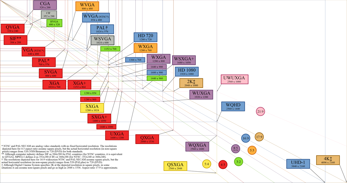
(Fig.01 - Picture Resolutions, Source: Wikimedia Commons)
The amount of pixels that are physically present in the actual LCD panel, or on a DLP chip in projectors, is called the native resolution. If the source video content doesn’t match the native display resolution, it has to be scaled up or scaled down to fit the screen. Scaling of a video signal will always have an impact on the image quality, as some pixel information has to be either removed or interpolated.
Aspect Ratio
The aspect ratio of an image describes the proportional relationship between its width and its height. The most commonly known aspect ratio nowadays might be the 16:9 (Widescreen) format. For example, a projection surface which is about 9ft high, has to be at least 16ft wide to accommodate for a picture in 16:9 format. Another way of stating the aspect ratio is to divide the screen width through the height. For a 16:9 display this will be 16/9 = 1.78, or also called 1.78:1
Commonly used aspect ratios:
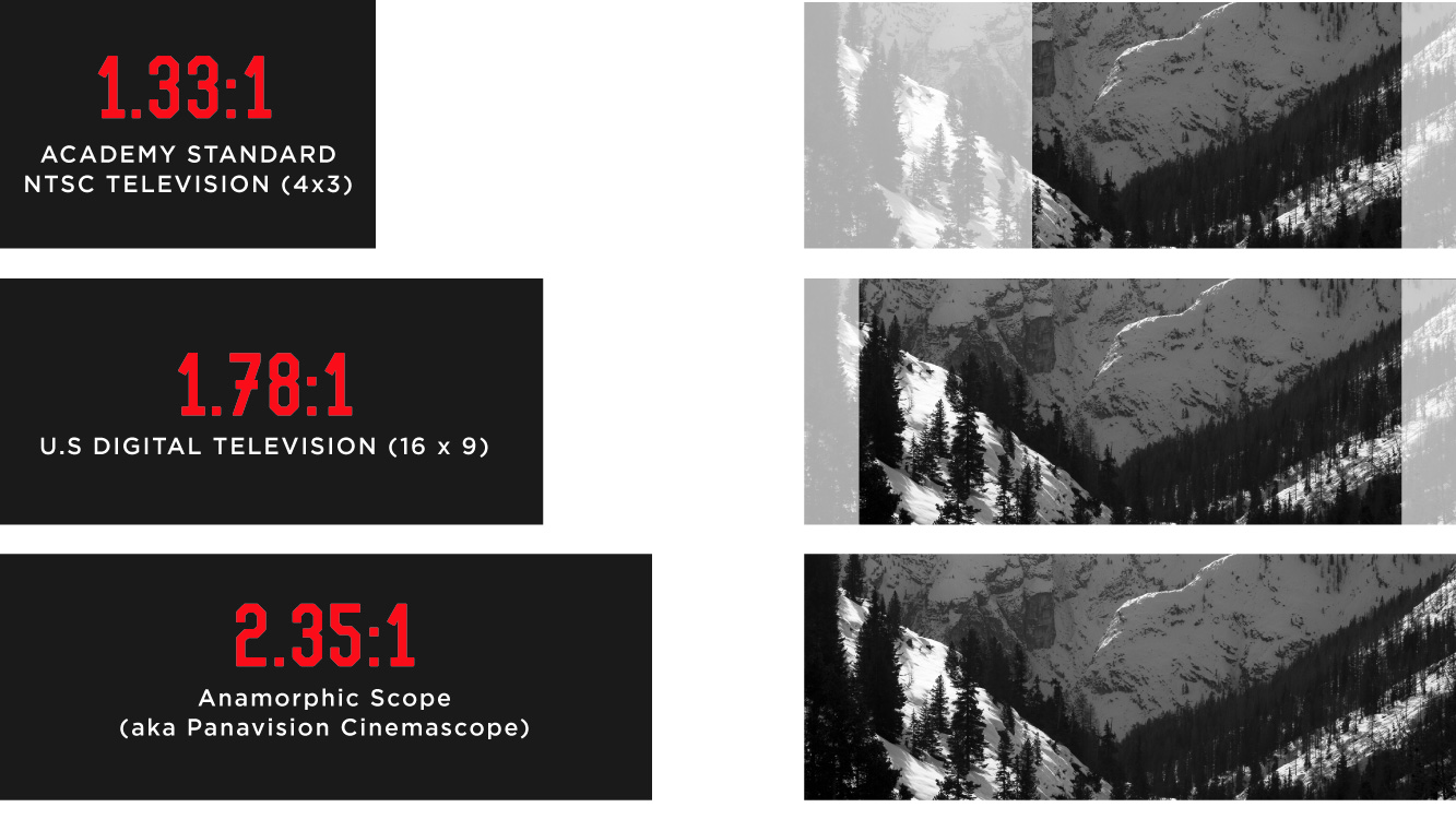
(Fig.02 - Common Aspect Ratios)
Color Sampling
Color Bit-depth
Color bit-depth is a binary number which represents the total number of possible values for each color component. Much like in digital audio, the more bits we have the greater depth possible for the signal. (examples: 10-bit, 12-bit). Note that this refers to the number of bits for "one" of the three components that make up the total color space. You will often see color bit-depth referred to as 24-bit True color or 36-bit Deep color. These refer to sum of bits used for all color components of a single pixel. For example, using RGB and 8-bits per component is what is used to make up the expression 24-bit True color (8 bits for red, 8 bits for green, 8 bits for blue, equals 24 bits total). 12-bits per component (times our three components) results in 36-bit Deep color. While these are two different meanings for the same term, it is unfortunately how these terms are often expressed. For the rest of this article when we refer to color bit-depth, we are referring to the bit-depth of each component and not the sum of the three components.
RGB Color Model
The color of an individual pixel in the RGB color model is described by indicating how much of each of the red, green, and blue is included. The color is expressed as an RGB triplet (r,g,b), each component of which can vary from zero to a defined maximum value. If all the components are at zero the result is black; if all are at maximum, the result is the brightest representable white. To create the color information of an individual pixel in 24-Bit colors, every color is expressed by an 8-bit byte, which can be represented by a decimal number ranging from 0 to 255.
A good example for additive RGB color mixing, is the typical color picker tool used in many PC software to set a custom color tone:
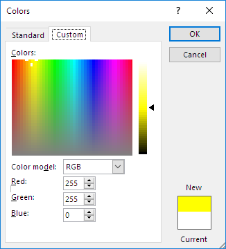
(Fig.03 - Microsoft Word Colorpicker)
Yellow: 255; 255; 0 // White: 255; 255; 255 // Red: 255; 0; 0 // Cyan: 0; 255; 255
RGB will always express the full color value and can be considered to be a 'raw' or uncompressed type of color format, which requires a lot of bandwidth in transport. By design, it won't natively support color subsampling and needs 3rd party compression algorithms to reduce its bandwidth.
Y'CbCr Color Model
In the Y'CbCr color model, the three colors Red, Green, and Blue are not expressed as an individual value like it is done in RGB. Instead, the information will be encoded into a luminance value (Y) and two chrominance components (Cb, Cr)
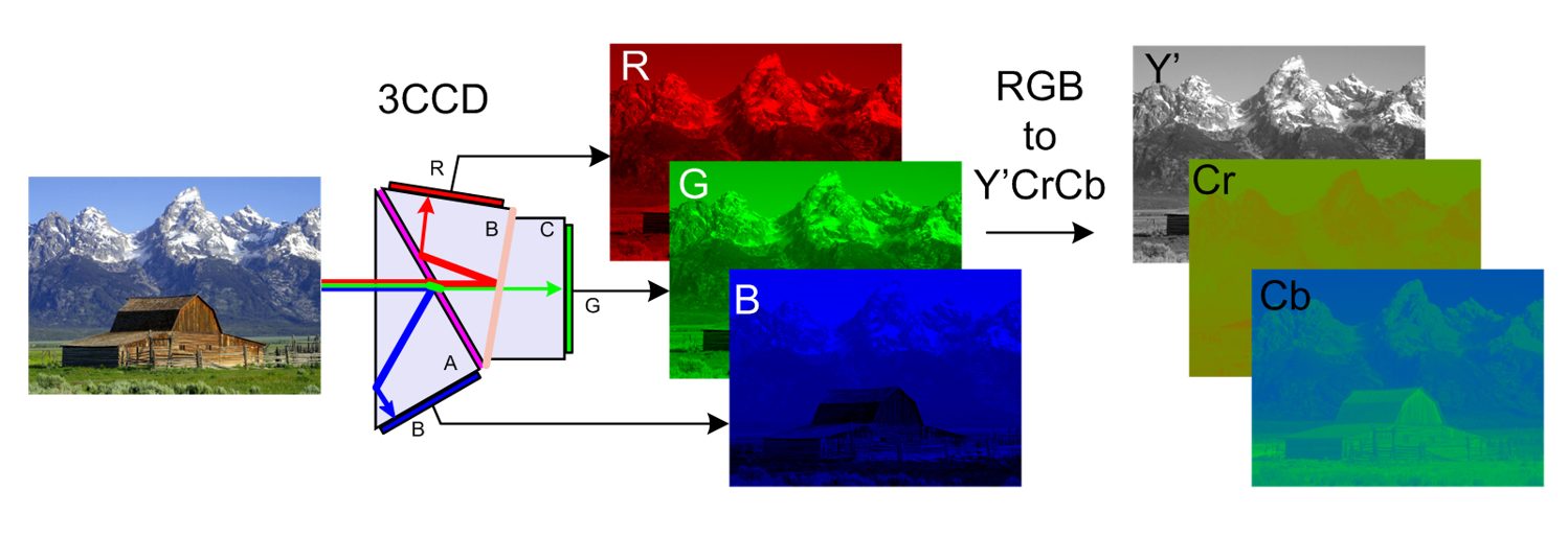
(Fig.04 - RGB/YCbCr Color Sampling, Source: Wikimedia Commons)
Basically, Y'CbCr color sampling is the digital version of its analog predecessors Y'UV and Y'PbPr. Often times all of these color models, which are very similar to how colors are encoded in the original RGB information, are summarized under the name YUV. From its origin, the Y′UV color model is used in the PAL and SECAM composite color video standards. Previous black-and-white systems used only luma (Y′) information. Color information (U and V) was added separately via a sub-carrier so that a black-and-white receiver would still be able to receive and display a color picture transmission in the receiver's native black-and-white format.
Besides its backwards compatibility to older viewing systems, which would be quite irrelevant nowadays, the Y'UV color sampling method has another advantage compared to RGB. It allows for down-sampling the color information in order to save storage space and video bandwidth on the wire.
Chroma Subsampling
Chroma Subsampling is a method to reduce the amount of data information of a Y'CrCb video signal. The perception of the human visual system (HVS) is less sensitive to color information than it is to changes in luminance, or brightness. So even if the human vision is capable of resolving differences in luminance in fine detail, it may not recognize if chroma information is greatly reduced in the resulting picture. Basically, a video signal that takes advantage of Chroma Subsampling will use less bandwidth because the color information in the signal has a lower resolution than the brightness information.
So the result is a lower bandwidth footprint due to fewer bits per pixel, at the cost of image detail. Chroma Subsampling specifications are expressed as a three digit ratio and are applied over a 4 x 2 block of pixels. Some examples are 4:2:0, 4:4:4, and 4:4:2. Let's look at an example of how a ratio of 4:2:2 would be applied to a pixel encoded in YUV. The Y' luminance component is represented by the 4:2:2. This means each row retains all 4 pixels worth of data. Or in other words, we don't discard any information for luminance for either row of 4 pixels. The second two numbers 4:2:2 means that for each row of 4 pixels, only 2 pixels of data are stored for both U and V. In other words, one pixel must be shared for every two pixels. This will be true for both the U and V components. This essentially cuts the amount of data we need in half for each U and V component since we are sharing one pixel's data for every two pixels. This will have a small impact on image detail but with a significant gain in reducing the amount of data required over the entire image.
Here is a visual example of how these ratios get applied:
Encoding scheme = J : a : b
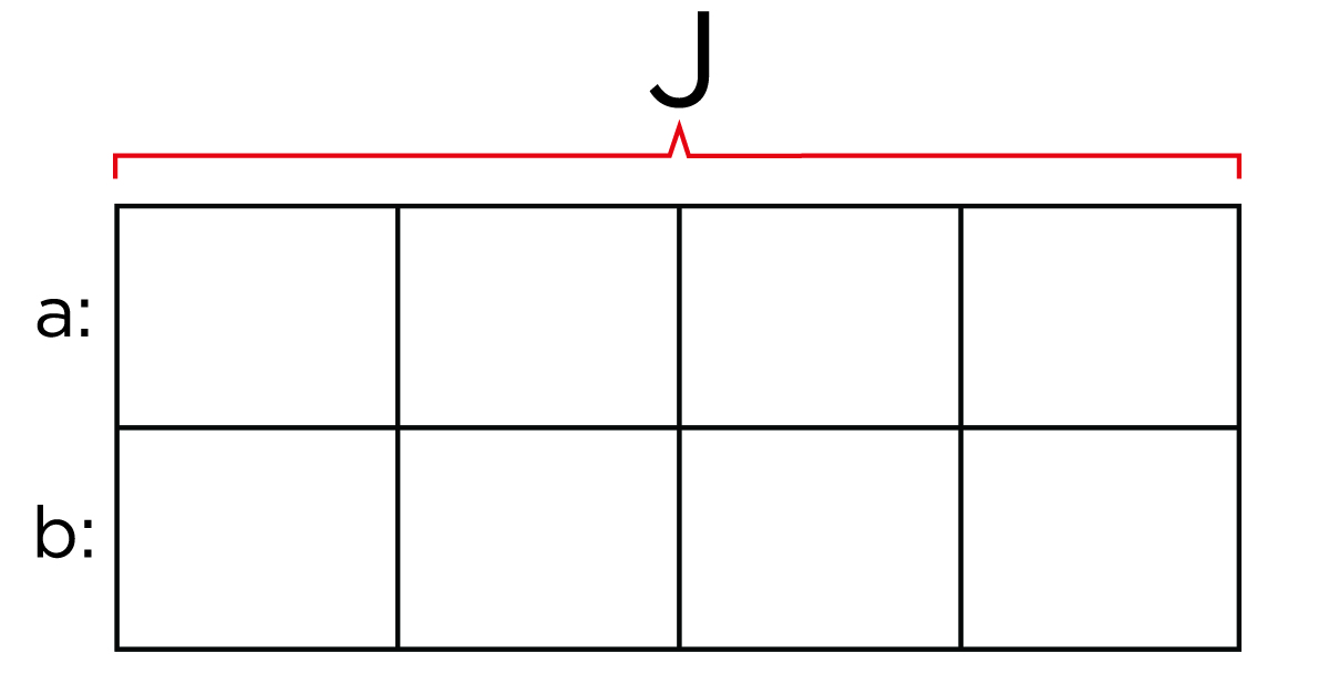
(Fig.05 - 4:4:4 Encoding grid with 2 lines and 4 rows)
J = Reference Block Size (Width, # of Columns)
- The Height or # of Rows is fixed at 2
a = Number of pixels in 1st row that get a sample
b = Number of pixels in the 2nd row that get a sample
In terms of bandwidth reduction, 4:4:4 sampling will provide full color reproduction and therefore won't reduce the video bandwidth - it requires the same data like an image formatted in RGB. An image sampled in 4:2:2 reduces the color information by half, while 4:2:0 and 4:1:1 only uses 1/4 of the original color information. For example, Ultra-HD Blu-Ray discs are encoded at 4:2:0 and produce a very high image quality.
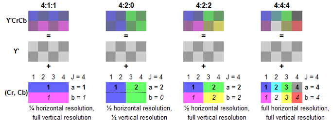
(Fig.06 - Examples of different color sampling formats)
Frame Rate
The frame rate of a video signal defines how many consecutive images will be displayed in a finite amount of time, to result in a motion picture perception at the viewer. Usually the frame rate is expressed in frames per second (FPS).
Good examples are the two major television standards NTSC and PAL, which are referring to a frame rate of 30 FPS (NTSC) and 25 FPS (PAL). Those frame rates originated from the frequency of the mains power supply in the counties in which each standard has been established. Modern theatrical film runs at 24 FPS. This is the case for both physical film and digital cinema systems.
As digital video has become more popular in consumer electronics and professional applications, not only did the image resolutions increase to higher definition content, but the frame rates of displays have also improved. One reason for higher frame rates was due the fact that the average screen size got bigger, and a large picture with a high frame rate (>100 FPS) has far less visual flicker that could be noticeable through the viewer. However, still most of the video content is not natively produced in such high frame rates, which requires frames to be displayed multiple times on a modern video display.
A video format is often expressed as [resolution] followed by the scan mode and its [frame rate] like: 1080i 60Hz the “i” in this example indicates an “interlaced” image scan. Besides interlaced there is also another method, known as “progressive” scan.
- Interlaced: In the first frame, only the odd numbers of vertical lines are displayed, the even lines stay blank. In the following frame, the even numbers of vertical lines will be displayed, while the odd lines stay blank. This method effectively halves the required bandwidth and reduces flicker. Also it allows for better adaption of different frame rates, as overlapping frames can be merged into each other.
- Progressive: Each frame carries the full amount of vertical lines and the full image information is displayed on every single frame. Whilst requiring more video bandwidth, it will allow for better image quality compared to the interlaced method.
EDID
Extended Display Identification Data (EDID) is a mechanism for allowing a video source device to discover the capabilities of a display or rendering device. EDID data resides in the source and is typically made available over the display interface connection (HDMI, DP, DVI…). EDID began as a means to achieve “plug and play” when connecting a monitor of one manufacturer to a computer or graphics driver from another manufacturer.
This is a very straight forward procedure if there is just one source and one display, but with a larger number of input sources and displays involved in a system, EDID may cause some challenges:
A display presents its EDID information to a connected source to make it aware of its preferred resolution, frame rate, what other resolutions and frame rates it's capable of, and possibly other information such as speaker configuration or other details. The source then has the option to simply pass along its signal in the event the preferred display resolution matches, attempt to scale the signal to the display's preferred resolution, or agree upon an alternative format. The challenge for any video distribution system is in how to deal with variances in EDID if there are several different displays, but just one source signal. In worst case this will result in displays going dark or result in a less than ideal image configuration.
Hence most manufactures of video switching and distribution devices have added EDID management to their products for quite some time. There have been even products manufactured who's sole purpose is to solve problems introduced by EDID when multiple devices are in a system.
Video over Ethernet
The most important concept to understand about sending digital video over a network is how much data can potentially be involved.
In contrast, if we look at digital audio, there are basically three factors to be considered: The number of audio channels, the bit-depth of each channel, and the sampling frequency. A classic example is CD quality audio. 2 channels, sampling frequency of 44.1khz, and a bit-depth of 16 bits. This translates to 1.4Mbps of data to represent the audio signals.
In a single digital video signal, there are 5 relevant factors to determine how much data is required:
- Video Resolution - Which is the size of the digital video image - (examples: 4k, 1080p, 720p, etc... )
- Frame Rate - The speed at which the digital image is refreshed - (examples: 60hz, 30hz, etc... )
- Color space - The gamut of possible colors that can be represented by the color encoding of a signal. (examples: RGB, YUV, Y'CrCb)
- Chroma Sub-sampling - The reduction of color information by using fewer bits per pixel at a cost of color space. (examples: 4:4:4, 4:2:2, 4:2:0)
- Color bit-depth - This is the binary number which represents the total number of possible values for each color component. In much like digital audio, the more bits we have the greater depth possible for the signal. (examples: 10-bit, 12-bit).
Let's take one example of an uncompressed video signal that is a common signal format:
1080p, 60 Hz, YUV 4:2:2, 10-bit = 2.49 Gbps
We can read this line as a combination of all of the parameters we have shown above. If we were to break this statement out into a series of sentences, we read this as a digital video signal that has a resolution of 1080p with a frame rate of 60Hz. It utilizes the YUV color space and 4:2:2 chroma sub-sampling for each YUV component. There are 10-bits used for each of the three color components listed.
To calculate the bandwidth we start with the resolution of the image:
1920 * 1080 (for 1080p) = 2,073,600 pixels in an image of this size.
Then multiply by the refresh rate:
2,073,600 * 60Hz = 124,416,000 total pixels (per second)
You can think of this number 124,416,000 as the number of pixels a display will have shown in one second of video.
Now we need to remember that each pixel is made up of three components, each of them are of a certain bit depth. Furthermore we might be "sub sampling" a set of pixels to help reduce the data footprint with a small trade off in image detail.
We start with the Chroma subsampling ratio of 4:2:2. This ratio is applied over a 2 x 4 block of pixels or a total of 8 pixels as we previously learned. Thus we first need to take our total number of pixels and divide them by 8:
124,416,000 pixels / 8 pixels in our 2x4 row = 15,552,000 blocks of 8 pixels.
Now we calculate what we know regarding our Chroma subsampling ratio and apply that to the number of blocks making sure to include our 10-bit color bit-depth per component:
Y' = 8 pixels * 10-bits = 80 total bits for Y' for each 8 pixel block
U = 4 pixels * 10-bits = 40 total bits for U for each 8 pixel block
V = 4 pixels * 10-bits = 40 total bits for V for each 8 pixel block
Now we add those all together and multiply that against the number of blocks to finally arrive at the total amount of data required for this video signal:
160 bits for each 8 pixel block * 15,552,000 blocks = 2,488,320,000 total bits required for one second of video.
Or more nicely expressed: 2.49 Gbps
To further illustrate how bandwidth-intensive video data is, it can be compared to the amount of data required for a channel of digital audio. Biamp uses 24-bit 48000Hz for digital audio data in Tesira:
24 * 48000 = 1.15Mb required for once second of audio.
In place of our one video signal described above, we could instead have 2,160 audio channels!
Examples of various video formats
After changing a few parameters in the equation of our example signal above, 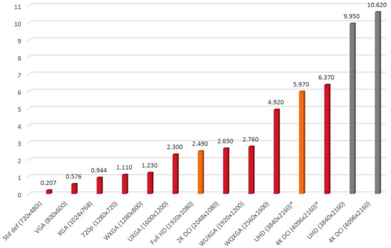
we will see what a difference it makes in terms of data bandwidth:
1080p, 60 Hz, YUV 4:2:0, 10-bit = 1.87 Gbps
1080p, 60 Hz, YUV 4:4:4, 10-bit = 3.73 Gbps
1080p, 60 Hz, RGB 4:4:4, 10-bit = 3.73 Gbps
1080p, 60 Hz, YUV 4:2:2, 8-bit = 1.99 Gbps
1080p, 30 Hz, YUV 4:2:2, 10-bit = 1.24 Gbps
2160p, 60 Hz, YUV 4:2:2, 10-bit = 9.95 Gbps
(Fig.07 - Bandwidth comparison of different video formats)
Compression
Even though a high throughput AVB network infrastructure is capable of real-time, uncompressed video transport, the video data bandwidth it is going to accommodate can be huge. When running very high resolutions and frame rates, like 4K @ 60Hz, a physical network link may reach its bandwidth limits with just one video stream. However, there will be applications that demand for transport of multiple video streams through the same pipe. In order to compensate for that, the video content may be compressed.
There is a variety of compression codecs available, and all of them work in a very similar way: they either leverage image redundancies within one frame, or throughout a series of frames. In the last 20 years, gains in video compression have increased about 400 percent, but over that same period, the complexity of the algorithms has increased one hundred-fold (10,000%). This creates longer compression encode and decode times, resulting in increased system transmit latency. More recently developed algorithms focus primarily on high compression ratios, like those found in h.264/AVC or h.265/HEVC that are necessary for delivering video via internet and mobile networks. In those situations, latency is not a critical factor and even compression artifacts are being tolerated due to the given application.
In the field of professional video distribution, we have to be aware that only 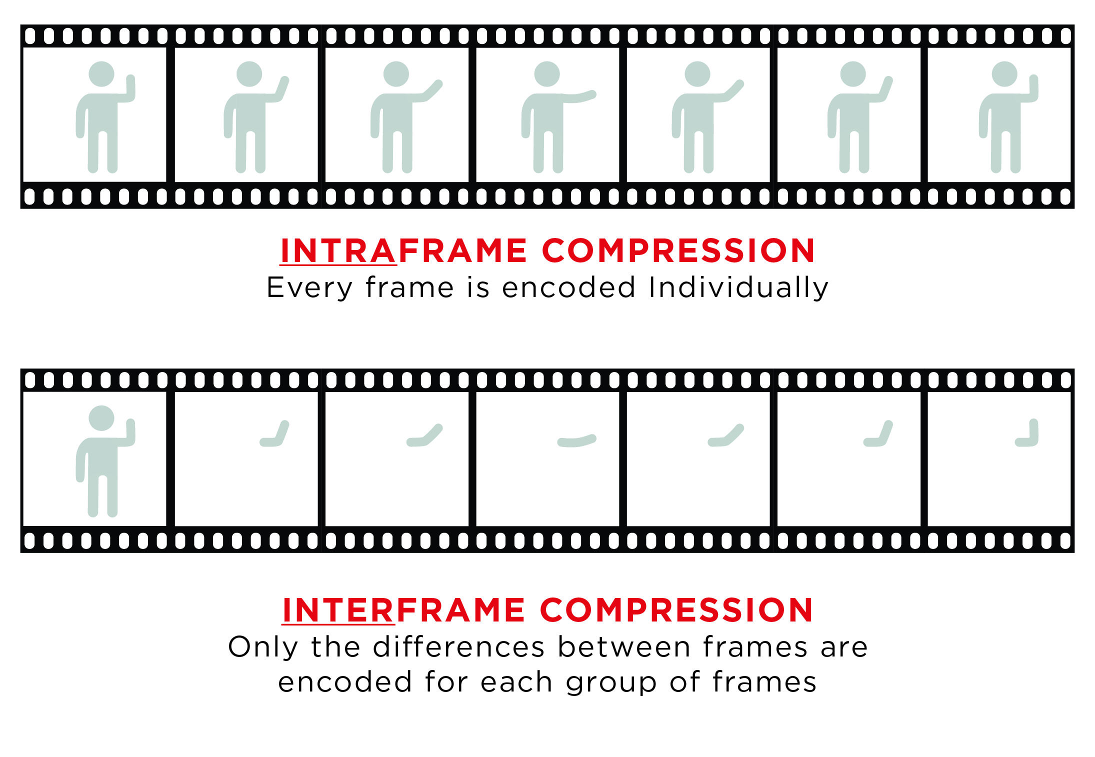 a few video codecs will qualify for “visually lossless” and low-latency transport. This being considered, the latest algorithm may not be the greatest.
Motion JPEG (M-JPEG) would be a good example here:
While most current algorithms use inter-frame compression (a.k.a. interframe prediction), for which a series of frames are being compressed in one sequence, M-JPEG in an intra-frame compression scheme, applied to every single video frame individually. On one hand this leads to relatively low compression ratios, but it allows for faster encoding times while the visual compression loss is kept at a minimum.
A word about codec latencies:
In a local area video deployment, multiple displays presenting the same content may be visible from one viewing position. It goes without saying that all those displays shall be in sync to each other. Long latencies will drive up the overall transmission latency of the whole system, as in time aligned systems, the longest run will set the reference. That makes it very important to use a fast, low-latency video compression algorithm.
(Fig. 08 - Intraframe vs. Interframe compression method)
Comparison of commonly-used compression codecs
|
Intra-Frame Compression:
|
Interframe Compresseion:
|
|
|
M-JPEG, JPEG 2000 (Spatial) |
MPEG-4, H.264 (Temporal) |
|
Latency Bandwidth Compression Processing Error Tolerance |
As low as 33 msec High < 25:1 Symmetric High |
200 msec or higher Low > 25:1 Asymmetric Low (Reference Frames) |
Compression affecting image quality
Based on the example of Motion JPEG, compression ratios up to 2:1 (50% bandwidth reduction), can be considered "mathematically lossless". This term basically describes that after a full encoding and decoding process, the image can be restored to its original specifications without losing any data information. Compression ratios up to 6:1 are still considered "visually lossless", so the decoded image output presented on a display reveals no visible difference to the original, uncompressed content. At higher ratios (>10:1) visually detectable artifacts may occur. However it should be mentioned that the human eye is unlikely to spot compression artifacts on any motion picture content, hence still image compression is more critical.
Some common image compression artifacts are classified as:
- Blocking – Regular structure (8x8 pixels) from block based algorithms
- Blurring – Loss of high frequency content (fine details and sharp edges) from quantization choices
- Ringing – Echo/ halo from filtering, present on steep edges
- Mosquito Noise – time variant prediction errors/ flickering or "edge busyness" in high frequency content
Example of visual artifacts:
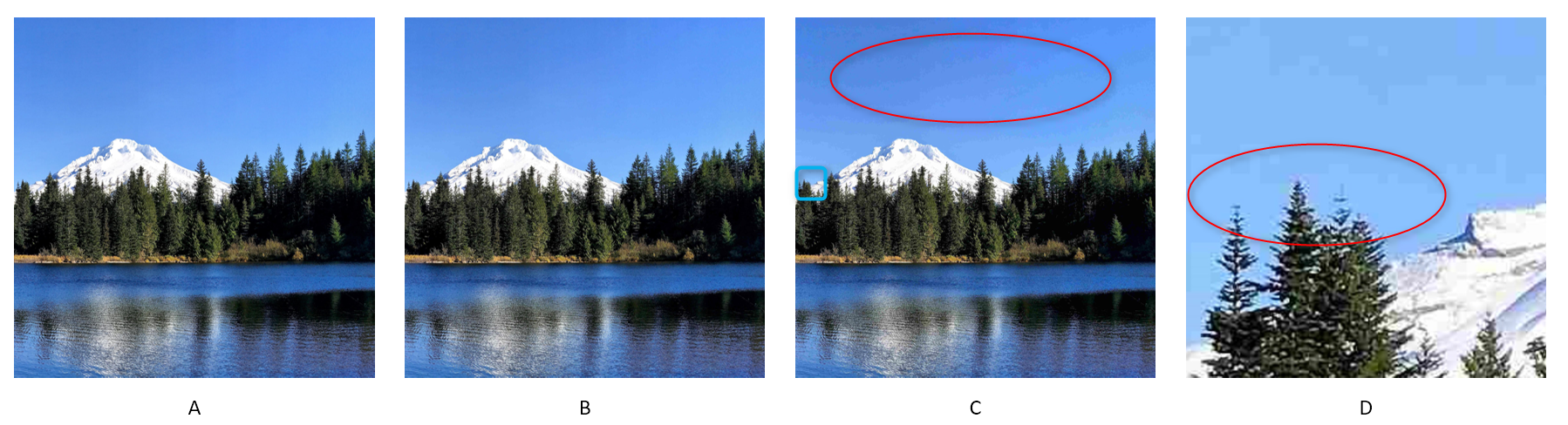
(Fig.09 - Visual example of compression loss)
The sample image is saved at progressively higher compression levels, starting at 1:1 (a), then 3:1 (b), then 10:1 (c). Even at 10:1, the image remains very legible, though obvious visual artifacts are present. The last picture (d) shows the 10:1 compressed image when zoomed at 10x. There is obvious smudging of detail, as well as a “blocking” artifact - a key characteristic of the JPEG lossy compression format.
HDCP
HDCP stands for: High-bandwidth Digital Content Protection and is a specification developed to protect entertainment content across digital interfaces. The standard is owned and maintained by DCP (Digital Content Protection LLC), a subsidiary of Intel™ Corporation. Its purpose is to prevent HDCP-encrypted content from being decoded and played on unauthorized devices. In the most basic configuration, an HDCP source device will check if the display is HDCP authorized. If it is authorized the devices perform a key exchange to create an encrypted path from source to display. This is usually all fine and good if we are talking about a single source and a single display. Even in this most basic scenario problems can arise. As we will learn in this lesson, one must take care with ensuring HDCP will function properly when several devices across a network are involved.
HDCP Versions
HDCP 1.0 came out when DVI (Digital Visual Interface) was first developed and released in the year 2000. HDCP 1.0 was improved upon and revised up until 2009, ending with HDCP 1.4. Other interface formats such as HDMI helped drive the development.
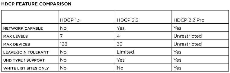
The HDCP 1.x versions allows up to 128 devices and up to 7 levels. HDCP 1.x devices each have their own unique key and when source attempts to interface with a sink, a key exchange is performed to create the secure channel.
HDCP 2.0 was released around 2008, as a successor to HDCP 1.x. It added more features such as the ability to support compressed signals, locality checking, and was based on TCP/IP which made it network capable. HDCP 2.0 was also developed because the cryptography methods used in 1.x versions had been compromised for some time by this point. It wasn't long before the same happened to version 2.0 and thus HDCP versions 2.1 and eventually 2.2 were developed. The subsequent versions of HDCP 2.x were also developed due to the protocol's encryption being exploited. And with the most recent version of "2.2 for HDMI" and "2.2 for MHL" released in early 2013, these versions are not backwards compatible with other 2.x versions. The method in which HDCP compliance is checked also changed in 2.0. Source devices maintain a "Global constant" key and each sink device carries a unique Receiver ID.
These HDCP 2.2 versions allow up to only 32 devices and a total of 4 levels deep. Note that the device count includes any individual device in the chain be it a source, repeater, or a sink. That means, if there will be a 33rd device or a non-HDCP 2.2 compliant device is added to the system, then all devices in the system will be aware that there is a non-compliant path as part of the system and all the displays will cease displaying the content!
It is also worth mentioning that if a device leaves or joins the system it causes the entire system to re-initialize the HDCP compliance checking process. This means that of all displays will be shortly interrupted until every devices has been confirmed to be HDCP compliant.
HDCP 2.2 Professional
In order to address the problems that arise for professional A/V systems, there is also another HDCP 2.2 version on the way to help address these limitations and behaviors. HDCP 2.2 Pro will provide an unrestricted number of devices to exist in a system. It will also allow an unrestricted number of levels in a system. Device leaving/joining the network will also be more robust in HDCP 2.2 Pro and will not cause the entire network to check that all devices are in compliance.
HDCP 2.2 Pro describes a “Pro Repeater” function that carries this ability to have an unlimited number of downstream devices, both HDCP 1.x and 2.2 capable. Pro devices must carry a label declaring that they have limited distribution and must not be re-deployed. What this means is that once it's installed, it cannot be used anywhere else!
The Pro Repeater carries a System Renew-ability Message file (SRM). This is a file with a list of revoked device IDs. As you might assume, this means if a device is on this list it will not receive protected content. Pro devices require Licensed Installers to report each repeater location at time of sale. After a Pro Repeater has been installed the SRM file will only be valid for a specific amount of time. It will be required for the Licensed Installer to update the SRM file before it expires. This will likely need to happen on an annual basis.
Connectors
There are a variety of digital video connectors out there. SDI, HDMI, DisplayPort, DVI, USB, MHL, Lightning and all of the mini and micro form factors in between. HDMI and DisplayPort are the most widely implemented standards. HDMI is dominant in video electronics while DisplayPort has replaced DVI for computers. The good news is that HDMI, DisplayPort and DVI are all based on the same video mode standards and can be easily adapted from one to another.
HDMI
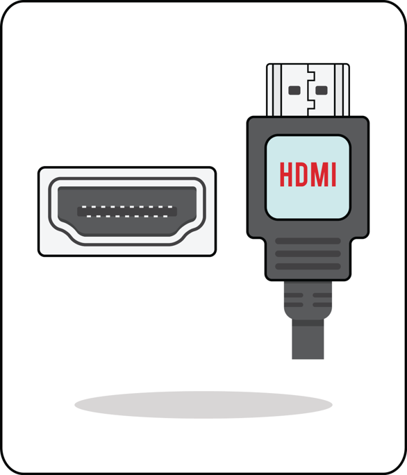
The 'High Definition Multimedia Interface' which has been released to the consumer AV market in 2003, has been constantly improved to accommodate for higher video bandwidths. While its first revision 1.0 supported a data rate of 3.96GB/s and video resolutions up to 1080p, a more recent generation like HDMI 2.0a provides a data throughput up to 18GB/s to provide features like 4K resolution, 3D and HDR video content. HDMI was originally designed for the consumer market but it became a common standard in majority of video hardware also in the semi-professional market. HDMI connectors have no locking mechanism, which is a potential cause of failure due to improperly plugged connections.
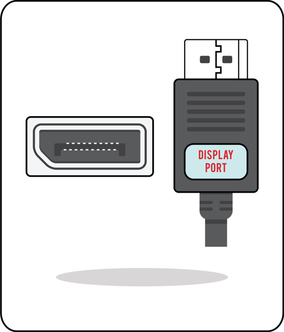
DisplayPort
Developed by VESA, the DisplayPort interface was and released in 2007 to mainly target the market of computer video interconnections. The release of variations like the mini- and micro DisplayPort, with a much smaller form factor, made it suitable for compact mobile devices like small laptop computers and netbooks. From its first revision DP 1.1, it has been designed to support HDCP content protection and data rates up to 5.2GB/s. DisplayPort also supports multiple video streams, up to four so-called 'lanes'. This allows for multiple displays to be daisy-chained together. The availability of a mechanical locking mechanism for DisplayPort connectors helped them becoming the connector of choice in commercial applications. The overall specifications are relatively similar to HDMI, however DisplayPort in native mode lacks some HDMI features such as Consumer Electronics Control (CEC) commands, which allow the control of multiple devices through a single remote.